Hong Kong Accreditation Service (HKAS) arranged "Analytical Quality Training Programme" from 9 to 13 Jan 2012. LGC experts were invited to provide this training. LGC is the UK’s designated National Measurement Institute for chemical and biochemical analysis , the National Reference Laboratory for a range of key areas, and is also the host organisation for the UK’s Government Chemist function.
The first day training topic was "Statistics for Analytical Chemists" and I was pleasure to be one of participants in the training. The training content was summarized for sharing.
In the beginning, Dr. John Ho (Accreditation Office, HKAS) introduced the two speakers. They were Dr. Stephen Ellison and Ms. Vicki Barwick from LGC.

Dr. Stephen Ellison presented the first topic entitled "Introduction to statistics". He introduced some fundamental statistic concept such as population, sample, distribution, mean, standard deviation, confidence intervals, etc.

He explained in general that the degrees of freedom is the number of data points (n) less the number of parameters already estimated from the data. (v = n - 1)

The concept of relative standard deviation (rsd) was introduced which also call coefficient of variation (CV). rsd = CV = s / ū
Then he also briefed the standard deviation of the mean (sdm) that the number of observations in each 'sample' increases, so the sdm values becomes smaller. It formed an estimate of the uncertainty of the mean value.

The second part speaker was Ms. Vicki Barwick and she introduced Significance Testing - Difference involving mean values: The t test.

She mentioned the two particularly common tests were called t and F, and were used for testing means and standard deviations respectively. There were 8 significance testing procedures below.
1. State the question
2. Select the correct test
3. Choose a level of significance (usually α = 0.05)
4. Decide number of tails
5. Calculate degrees of freedom from the data
6. Look up the critical value
7. Calculate the test statistic from the data
8. Compare test statistic with critical value or inspect 'p-values'

The follow diagram showed the decision of one-tailed or two-tailed for different hypotheses.

The Ms. Vicki Barwick introduced two types of t test for comparing means. The following form is valid only if the two data sets have similar standard deviations.

In the following diagram, the paired sets of results used the paired-t test that t was calculate using the mean difference. In each pair, the different coloured circles could represent different treatments, different method, or a different time, analyst or other change.

And then Dr. Stephen Ellison explained the F-test.

We used the F-test to comparing spread. The spread of sets of data were compared to:
1. Decide whether a difference in spread is real, or just a product of random variation
2. Decide whether two data sets really could be looking at the same thing

The following diagram showed the rules for the F-test. For one-tailed test, it is for s1^2 > s2^2; there is no need to carry out the test if s1^2 < s2^2. For two-tailed test, put the largest variance on the top line of the ratio to calculate F.

After lunch, Dr. Stephen Ellison demonstrated why use of ANOVA and some participants were invited to help for this demonstration.

The ANOVA table was explained that the Sum of Squares (SS) included Between Groups (b), Within Groups (w) and Total (tot).
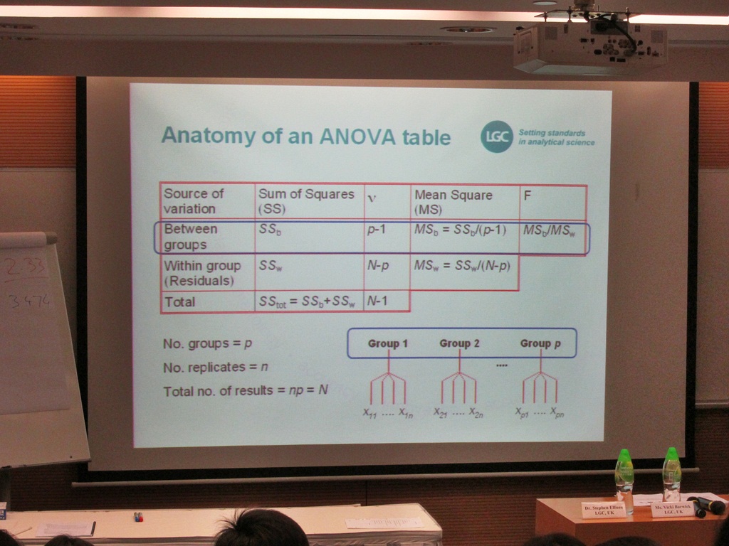

The following diagram showed SS(b) = SS(tot) - SS(w), where F = MS(b)/MS(w). It uses one-tailed test and F>F-crit means the differences between groups of data are significant compared to within group variation.
In one-way ANOVA,
the null hypothesis (H0) is: There is no different between the within group Mean Square (MS) and the between groups MS.
the alternative hypothesis (H1) is: The between groups MS is greater than the within group MS.

Lastly, Ms. Vicki Barwick mentioned Linear Regression which used to establish or confirm a quantitative relationship (e.g. Calibration) and to find out whether a linear relationship exists.

Then She brief the 5 general procedures of linear regression step by step.
1. Inspect the data and scatterplot
2. Calculate the fitted line
3. Inspect the residuals
4. Inspect the regression statistics
5. Calculate the predicted values and their confidence limits

The residual plots were useful to interpret the nature of data such as curved response and showed below.

The following diagram is used for interpreting the correlation coefficient (r). The significance of the r value depends on the number of data points used to calculate it. If absolute r value lying in the shaded region, it is to be considered statistically significant at the 95% confidence level.

At the end, the prediction interval of using linear regression was briefed.

Reference:
HKAS - www.hkas.gov.hk
LGC - http://www.lgc.co.uk/

沒有留言:
發佈留言